


Shiny is more than just an R package; it is a plat- form that revolutionizes the way analysts and sta- tisticians share their work. Developed by RStudio, this package allows complex statistical analyses to be integrated with interactive web interfaces, all within the familiar R environment. With no prior knowledge of web development required, R users can create applications that not only display re- sults but also allow users to manipulate data and parameters in real time.
Brief description of R
R is a programming language and software en- vironment specializing in statistical analysis and data visualization. Widely used by statisticians, data scientists and analysts, R offers an extensi- ble platform that supports various data handling operations, statistical calculations and graphics. Its ability to integrate code from other languages such as C, C++ and Fortran, and its open source nature, has made it popular in academia, research and industry.
Basics concepts of Shiny
Shiny clearly divides the user interface (UI) and the server logic:
UI.R: specifies how the web application will look to the end user. This user interface may include elements such as input controls (such as buttons, sliders, text boxes), graphics, tables, and any other interactive elements that the user may use to interact with the application.
Server.R: Executes the R code and processes the ap- plication logic, handling the inputs and generating the outputs.
Global.R: is an R framework for building interactive web applications. In a Shiny application, global.R is used to define variables, functions, and other elements that must be available on both the server and client sides of the application. This may include loading data, defining helper functions, and configuring global options.
Principal Components
ui.R: This user interface may include elements such as input controls (such as buttons, sliders, text boxes), graphics, tables, and any other interactive elements that the user may use to interact with the application.
server.R: Defines reactive functions that run in response to events, such as clicking a button or changing the value of an input control. These reactive functions can perform calculations, filter data, perform visualizations, and any other tasks necessary to update the user interface based on user actions.
global.R: is an R framework for building interactive web applications. In a Shiny application, global.R is used to define variables, functions, and other elements that must be available on both the server and client sides of the application. This may include loading data, defining helper functions, and configuring global options.
Requirements
R languague for Windows
RStudio Application
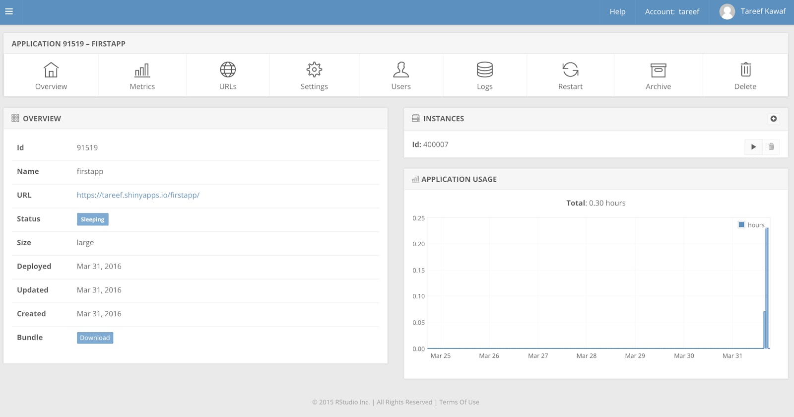
Installation of Shiny and RStudio
We install the R package for Windows from its official website. Once installed, we proceed to install RStudio also from its official website. Once everything necessary has been installed, we proceed to create 3 new scripts with the following names: ui.R, server.R and global.R.
Code for global.R
#### Load the required packages ####
# if packages are not installed already,
# install them using function install.packages(" ")

library(shiny) # shiny features
library(shinydashboard) # shinydashboard functions
library(DT)  # for DT tables
library(dplyr)  # for pipe operator & data manipulations
library(plotly) # for data visualization and plots using plotly
library(ggplot2) # for data visualization & plots using ggplot2
library(ggtext) # beautifying text on top of ggplot
library(maps) # for USA states map - boundaries used by ggplot for mapping
library(ggcorrplot) # for correlation plot
library(shinycssloaders) # to add a loader while graph is populating

#### Dataset Manipulation ####
# USArrests dataset comes along with base R
# you can view the data by simply
# USArrests  # uncomment if running this

## create a states object from rownames
states = rownames(USArrests)

## Add a new column variable state into the dataset. This will be used later to merge the dataset with US states map data
my_data <- USArrests %>%
  mutate(State = states)

# Column names without state. This will be used in the selectinput for choices in the shinydashboard
c1 = my_data %>%
  select(-"State") %>%
  names()

# Column names without state and UrbanPopulation. This will be used in the selectinput for choices in the shinydashboard
c2 = my_data %>%
  select(-"State", -"UrbanPop") %>%
  names()

####Preparing data for Arrests Map ####
# map data for US states boundaries using the maps package
# map_data from ggplot package
# map_data() converts data fom maps package into a dataframe which can be further used for mapping

state_map <- map_data("state") # state from maps package contains information required to create the US state boundaries
# state_map %>% str() # you can see that state_map has a region column. region column has US state names but in lower case


# convert state to lower case
my_data1 = my_data %>%
  mutate(State = tolower(State))  # converting the state names from USArrests dataset to lower case so we can later merge the maps data to our dataset


## Add the latitude, longitude and other info needed to draw the ploygon for the state map
# For the state boundaries available - add the USAArrests info.
# Note that Alaska and Hawaii boundaries are not available, those rows will be omitted in the merged data
# right_join from dplyr package
merged =right_join(my_data1, state_map,  by=c("State" = "region"))

# Add State Abreviations and center locations of each states. Create a dataframe out of it
st = data.frame(abb = state.abb, stname=tolower(state.name), x=state.center$x, y=state.center$y)

# Join the state abbreviations and center location to the dataset for each of the observations in the merged dataset
# left_join from dplyr package
# there is no abbreviation available for District of Columbia and hence those rows will be dropped in the outcome
new_join = left_join(merged, st, by=c("State" = "stname"))
Code for server.R
## Shiny Server component for dashboard

function(input, output, session){

  # Data table Output
  output$dataT <- renderDataTable(my_data)


  # Rendering the box header
  output$head1 <- renderText(
    paste("5 states with high rate of", input$var2, "Arrests")
  )

  # Rendering the box header
  output$head2 <- renderText(
    paste("5 states with low rate of", input$var2, "Arrests")
  )


  # Rendering table with 5 states with high arrests for specific crime type
  output$top5 <- renderTable({

    my_data %>%
      select(State, input$var2) %>%
      arrange(desc(get(input$var2))) %>%
      head(5)

  })

  # Rendering table with 5 states with low arrests for specific crime type
  output$low5 <- renderTable({

    my_data %>%
      select(State, input$var2) %>%
      arrange(get(input$var2)) %>%
      head(5)


  })


  # For Structure output
  output$structure <- renderPrint({
    my_data %>%
      str()
  })


  # For Summary Output
  output$summary <- renderPrint({
    my_data %>%
      summary()
  })

  # For histogram - distribution charts
  output$histplot <- renderPlotly({
    p1 = my_data %>%
      plot_ly() %>%
      add_histogram(x=~get(input$var1)) %>%
      layout(xaxis = list(title = paste(input$var1)))


    p2 = my_data %>%
      plot_ly() %>%
      add_boxplot(x=~get(input$var1)) %>%
      layout(yaxis = list(showticklabels = F))

    # stacking the plots on top of each other
    subplot(p2, p1, nrows = 2, shareX = TRUE) %>%
      hide_legend() %>%
      layout(title = "Distribution chart - Histogram and Boxplot",
             yaxis = list(title="Frequency"))
  })


  ### Bar Charts - State wise trend
  output$bar <- renderPlotly({
    my_data %>%
      plot_ly() %>%
      add_bars(x=~State, y=~get(input$var2)) %>%
      layout(title = paste("Statewise Arrests for", input$var2),
             xaxis = list(title = "State"),
             yaxis = list(title = paste(input$var2, "Arrests per 100,000 residents") ))
  })


  ### Scatter Charts
  output$scatter <- renderPlotly({
    p = my_data %>%
      ggplot(aes(x=get(input$var3), y=get(input$var4))) +
      geom_point() +
      geom_smooth(method=get(input$fit)) +
      labs(title = paste("Relation b/w", input$var3 , "and" , input$var4),
           x = input$var3,
           y = input$var4) +
      theme(  plot.title = element_textbox_simple(size=10,
                                                  halign=0.5))


    # applied ggplot to make it interactive
    ggplotly(p)

  })


  ## Correlation plot
  output$cor <- renderPlotly({
    my_df <- my_data %>%
      select(-State)

    # Compute a correlation matrix
    corr <- round(cor(my_df), 1)

    # Compute a matrix of correlation p-values
    p.mat <- cor_pmat(my_df)

    corr.plot <- ggcorrplot(
      corr,
      hc.order = TRUE,
      lab= TRUE,
      outline.col = "white",
      p.mat = p.mat
    )

    ggplotly(corr.plot)

  })


    # Choropleth map
  output$map_plot <- renderPlot({
      new_join %>%
      ggplot(aes(x=long, y=lat,fill=get(input$crimetype) , group = group)) +
      geom_polygon(color="black", size=0.4) +
      scale_fill_gradient(low="#73A5C6", high="#001B3A", name = paste(input$crimetype, "Arrest rate")) +
      theme_void() +
      labs(title = paste("Choropleth map of", input$crimetype , " Arrests per 100,000 residents by state in 1973")) +
      theme(
        plot.title = element_textbox_simple(face="bold",
                                            size=18,
                                            halign=0.5),

        legend.position = c(0.2, 0.1),
        legend.direction = "horizontal"

      ) +
      geom_text(aes(x=x, y=y, label=abb), size = 4, color="white")


  })


}
Code for ui.R
dashboardPage(

  dashboardHeader(title="Exploring the 1973 US Arrests data with R & Shiny Dashboard", titleWidth = 650,
                  tags$li(class="dropdown",tags$a(href="https://www.youtube.com/playlist?list=PL6wLL_RojB5xNOhe2OTSd-DPkMLVY9DfB", icon("youtube"), "My Channel", target="_blank")),
                  tags$li(class="dropdown",tags$a(href="https://www.linkedin.com/in/abhinav-agrawal-pmp%C2%AE-safe%C2%AE-5-agilist-csm%C2%AE-5720309" ,icon("linkedin"), "My Profile", target="_blank")),
                  tags$li(class="dropdown",tags$a(href="https://github.com/aagarw30/R-Shiny-Dashboards/tree/main/USArrestDashboard", icon("github"), "Source Code", target="_blank"))
                  ),


  dashboardSidebar(
    sidebarMenu(id = "sidebar",
      menuItem("Dataset", tabName = "data", icon = icon("database")),
      menuItem("Visualization", tabName = "viz", icon=icon("chart-line")),

      # Conditional Panel for conditional widget appearance
      # Filter should appear only for the visualization menu and selected tabs within it
      conditionalPanel("input.sidebar == 'viz' && input.t2 == 'distro'", selectInput(inputId = "var1" , label ="Select the Variable" , choices = c1)),
      conditionalPanel("input.sidebar == 'viz' && input.t2 == 'trends' ", selectInput(inputId = "var2" , label ="Select the Arrest type" , choices = c2)),
      conditionalPanel("input.sidebar == 'viz' && input.t2 == 'relation' ", selectInput(inputId = "var3" , label ="Select the X variable" , choices = c1, selected = "Rape")),
      conditionalPanel("input.sidebar == 'viz' && input.t2 == 'relation' ", selectInput(inputId = "var4" , label ="Select the Y variable" , choices = c1, selected = "Assault")),
      menuItem("Choropleth Map", tabName = "map", icon=icon("map"))

    )
  ),


  dashboardBody(

    tabItems(
      ## First tab item
      tabItem(tabName = "data",
              tabBox(id="t1", width = 12,
                     tabPanel("About", icon=icon("address-card"),
fluidRow(
  column(width = 8, tags$img(src="crime.jpg", width =600 , height = 300),
         tags$br() ,
         tags$a("Photo by Campbell Jensen on Unsplash"), align = "center"),
  column(width = 4, tags$br() ,
         tags$p("This data set comes along with base R and contains statistics, in arrests per 100,000 residents for assault, murder, and rape in each of the 50 US states in 1973. Also, given is the percent of the population living in urban areas.")
  )
)


                              ),
                     tabPanel("Data", dataTableOutput("dataT"), icon = icon("table")),
                     tabPanel("Structure", verbatimTextOutput("structure"), icon=icon("uncharted")),
                     tabPanel("Summary Stats", verbatimTextOutput("summary"), icon=icon("chart-pie"))
              )

),

# Second Tab Item
    tabItem(tabName = "viz",
            tabBox(id="t2",  width=12,
                   tabPanel("Crime Trends by State", value="trends",
                            fluidRow(tags$div(align="center", box(tableOutput("top5"), title = textOutput("head1") , collapsible = TRUE, status = "primary",  collapsed = TRUE, solidHeader = TRUE)),
                                     tags$div(align="center", box(tableOutput("low5"), title = textOutput("head2") , collapsible = TRUE, status = "primary",  collapsed = TRUE, solidHeader = TRUE))

                            ),
                            withSpinner(plotlyOutput("bar"))
                   ),
            tabPanel("Distribution", value="distro",
                     # selectInput("var", "Select the variable", choices=c("Rape", "Assault")),
                     withSpinner(plotlyOutput("histplot", height = "350px"))),
            tabPanel("Correlation Matrix", id="corr" , withSpinner(plotlyOutput("cor"))),
            tabPanel("Relationship among Arrest types & Urban Population",
                     radioButtons(inputId ="fit" , label = "Select smooth method" , choices = c("loess", "lm"), selected = "lm" , inline = TRUE),
                     withSpinner(plotlyOutput("scatter")), value="relation"),
            side = "left"
                   ),

            ),


    # Third Tab Item
      tabItem(
      tabName = "map",
      box(      selectInput("crimetype","Select Arrest Type", choices = c2, selected="Rape", width = 250),
                withSpinner(plotOutput("map_plot")), width = 12)


    )

)
    )
      )